| L | A | n | Deaths (Y=1) | Pr[Y=1 | A, L] |
|---|---|---|---|---|
| 0 (female) | 0 (untreated) | 8 | 0 | 0.0 |
| 1 (male) | 0 (untreated) | 2 | 1 | 0.5 |
| 0 (female) | 1 (treated) | 2 | 0 | 0.0 |
| 1 (male) | 1 (treated) | 8 | 4 | 0.5 |
Chapter 7: Confounding
In Chapter 6 we described causal diagrams and showed how to read independence relations from them using d-separation. We also identified three structural sources of bias—confounding, selection bias, and measurement bias—and introduced the backdoor criterion as the graphical condition for eliminating confounding. This chapter examines confounding in greater depth. We show that confounding is equivalent to the absence of marginal exchangeability, characterize it through the structure of the causal diagram, and relate the structural (graphical) definition to the traditional epidemiological criteria for identifying confounders. We close with an introduction to Single-World Intervention Graphs (SWIGs), which embed counterfactual variables directly in a causal diagram.
This chapter is based on Hernán and Robins (2020, chap. 7, pp. 77–92).
1 7.1 The Structure of Confounding (pp. 77–80)
In a marginally randomized experiment (Chapter 2), the treated and untreated groups have the same distribution of potential outcomes because treatment was assigned independently of any pre-existing characteristics. As a result, the crude association between treatment \(A\) and outcome \(Y\) equals the average causal effect:
\[\Pr[Y = 1 \mid A = 1] - \Pr[Y = 1 \mid A = 0] = \Pr[Y^{a=1} = 1] - \Pr[Y^{a=0} = 1]\]
In an observational study, however, the distribution of pre-existing characteristics typically differs between the treated and untreated. If some of those characteristics affect the outcome, the crude association will not equal the causal effect. This discrepancy is confounding.
1.1 A Hypothetical Example
Consider a hypothetical observational study of the causal effect of a cholesterol-lowering drug (\(A\): 1 = treated, 0 = untreated) on 5-year mortality (\(Y\): 1 = died, 0 = survived), where sex (\(L\): 1 = male, 0 = female) affects both treatment assignment and mortality. The hypothetical data for 20 individuals are shown below.
Within each sex stratum, the mortality rate is the same for treated and untreated individuals:
\[\Pr[Y = 1 \mid A = 1, L = 1] = \Pr[Y = 1 \mid A = 0, L = 1] = 0.50\] \[\Pr[Y = 1 \mid A = 1, L = 0] = \Pr[Y = 1 \mid A = 0, L = 0] = 0.00\]
Within strata of \(L\), the association equals the causal effect (null). But the crude (marginal) association is non-null:
\[\Pr[Y = 1 \mid A = 1] = \tfrac{4}{10} = 0.40 \neq \Pr[Y = 1 \mid A = 0] = \tfrac{1}{10} = 0.10\]
The crude risk difference of \(0.30\) is entirely due to confounding: males are more frequently treated (\(8/10\)) and have higher baseline mortality (\(0.50\)) than females.
Why confounding arises here:
Males (\(L = 1\)) are more likely to receive treatment (80%) and have higher mortality (50%), while females (\(L = 0\)) are less likely to receive treatment (20%) and have lower mortality (0%). Within each sex, treatment has no effect. But marginally, treated individuals have higher mortality than untreated individuals—not because of any causal effect of treatment, but because the treated group is disproportionately male.
The crude risk difference of 0.30 is entirely confounding bias; the true average causal effect is zero.
1.2 The Structural Definition
In the causal diagram framework, confounding arises when there is an open backdoor path from \(A\) to \(Y\). In the example above, sex \(L\) is a common cause of treatment \(A\) and mortality \(Y\):
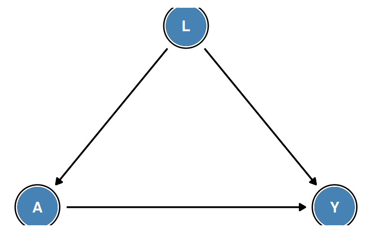
The path \(A \leftarrow L \rightarrow Y\) is a backdoor path from \(A\) to \(Y\). Because \(L\) is a non-collider on this path and has not been conditioned on, the path is open. Confounding bias exists whenever at least one backdoor path from \(A\) to \(Y\) is open.
Confounding can operate in any direction:
- Positive confounding: the crude estimate overstates the causal effect (or makes a harmful treatment look beneficial, or a beneficial treatment look even more beneficial)
- Negative confounding: the crude estimate understates the causal effect (or makes a beneficial treatment look harmful)
- The direction depends on the signs of the associations \(L \to A\) and \(L \to Y\)
In the drug example above, sicker patients (males) were more likely to receive treatment and had worse outcomes, so the drug appears harmful even though it has no effect. This is confounding by indication or channeling bias—the indication for treatment (higher disease severity) is itself a risk factor for the outcome.
2 7.2 Confounding and Exchangeability (pp. 80–82)
Confounding is mathematically equivalent to the failure of marginal exchangeability. Recall from Chapter 2 that marginal exchangeability holds when:
\[Y^a \perp\!\!\!\perp A \quad \text{for all } a\]
This means the treated and untreated groups have the same distribution of potential outcomes: \(\Pr[Y^a = 1 \mid A = 1] = \Pr[Y^a = 1 \mid A = 0] = \Pr[Y^a = 1]\).
When marginal exchangeability holds, association equals causation:
\[\Pr[Y = 1 \mid A = 1] - \Pr[Y = 1 \mid A = 0] = \Pr[Y^{a=1} = 1] - \Pr[Y^{a=0} = 1]\]
No confounding is equivalent to marginal exchangeability. When confounding is present, marginal exchangeability fails: \(Y^a \not\perp\!\!\!\perp A\), and the treated and untreated differ in their potential outcomes.
2.1 Eliminating Confounding via Conditioning
Even when marginal exchangeability fails, we can often achieve conditional exchangeability by adjusting for the measured confounders \(L\):
\[Y^a \perp\!\!\!\perp A \mid L \quad \text{for all } a\]
This means that within each stratum of \(L\), the treated and untreated are exchangeable. In the drug example:
- Within males (\(L = 1\)): \(\Pr[Y^{a} = 1 \mid A = 1, L = 1] = \Pr[Y^{a} = 1 \mid A = 0, L = 1]\) ✓
- Within females (\(L = 0\)): \(\Pr[Y^{a} = 1 \mid A = 1, L = 0] = \Pr[Y^{a} = 1 \mid A = 0, L = 0]\) ✓
Under conditional exchangeability and positivity, the standardization (g-formula) identifies the causal effect:
\[\Pr[Y^{a} = 1] = \sum_l \Pr[Y = 1 \mid A = a, L = l] \, \Pr[L = l]\]
Applying standardization to the data in Table 7.1:
\[\Pr[Y^{a=1} = 1] = 0.50 \times 0.50 + 0.00 \times 0.50 = 0.25\] \[\Pr[Y^{a=0} = 1] = 0.50 \times 0.50 + 0.00 \times 0.50 = 0.25\]
The standardized risk difference is zero, correctly recovering the null causal effect.
Marginal vs. conditional exchangeability:
- Marginal exchangeability (\(Y^a \perp\!\!\!\perp A\)): holds in marginally randomized experiments; association equals causation without any adjustment.
- Conditional exchangeability (\(Y^a \perp\!\!\!\perp A \mid L\)): holds in conditionally randomized experiments and (by assumption) in observational studies after adjusting for all confounders \(L\).
In practice, we can never verify from data alone that conditional exchangeability holds. We must rely on subject-matter knowledge to argue that the measured \(L\) captures all common causes of \(A\) and \(Y\).
The no-unmeasured-confounding assumption:
Conditional exchangeability given \(L\) is sometimes called the no-unmeasured-confounding assumption or ignorability. It is the key assumption required for identification of causal effects in observational studies.
3 7.3 Confounding and the Backdoor Criterion (pp. 82–85)
The backdoor criterion (Chapter 6) provides a graphical condition for identifying sets of variables \(L\) that suffice to eliminate confounding by adjustment.
3.1 Multiple DAG Structures
Different causal structures imply different sets of variables that satisfy the backdoor criterion.
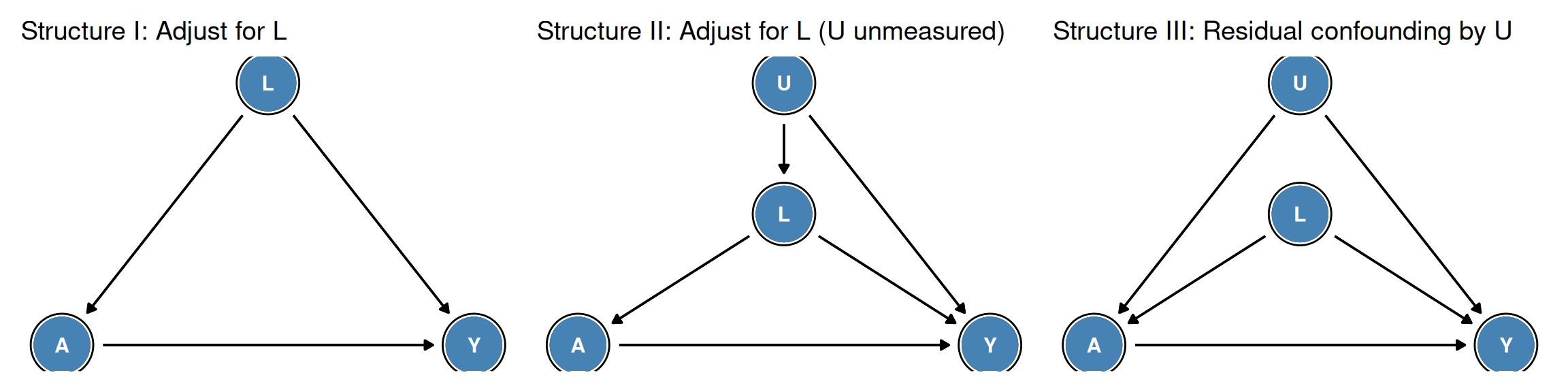
Structure I (\(L \to A\), \(L \to Y\), \(A \to Y\)):
- Backdoor path: \(A \leftarrow L \to Y\)
- \(\{L\}\) satisfies the backdoor criterion: \(L\) is not a descendant of \(A\) and blocks the only backdoor path.
- Adjustment for \(L\) suffices.
Structure II (\(U \to L \to A\), \(U \to Y\), \(L \to Y\), \(A \to Y\), \(U\) unmeasured):
- Backdoor paths: \(A \leftarrow L \to Y\) and \(A \leftarrow L \leftarrow U \to Y\)
- \(L\) is a non-collider on both paths; conditioning on \(L\) blocks them both.
- \(\{L\}\) satisfies the backdoor criterion: adjustment for \(L\) suffices even though \(U\) is unmeasured.
Structure III (\(U \to A\), \(U \to Y\), \(L \to A\), \(L \to Y\), \(A \to Y\), \(U\) unmeasured):
- Backdoor paths: \(A \leftarrow L \to Y\) and \(A \leftarrow U \to Y\)
- Conditioning on \(L\) blocks \(A \leftarrow L \to Y\), but the path \(A \leftarrow U \to Y\) does not pass through \(L\)—conditioning on \(L\) leaves it open.
- \(\{L\}\) does not satisfy the backdoor criterion because not all backdoor paths are blocked.
- Since \(U\) is unmeasured, no measured adjustment set can block \(A \leftarrow U \to Y\). The causal effect is not identified by adjustment alone.
Sufficient adjustment sets:
In Structure II, adjusting for \(L\) alone suffices even though \(U\) is unmeasured, because every backdoor path from \(A\) to \(Y\) passes through \(L\). This illustrates an important point: we do not need to measure all common causes; we only need to measure variables sufficient to block all backdoor paths.
In Structure III, the unmeasured \(U\) bypasses \(L\) entirely (direct arrow \(U \to A\)), so there is no measured set that can block the path \(A \leftarrow U \to Y\). This is unmeasured confounding that cannot be handled by standard adjustment methods.
Minimal sufficient adjustment sets:
Multiple different sets of variables may satisfy the backdoor criterion. A minimal sufficient adjustment set is one from which no variable can be removed while still blocking all backdoor paths. The R package dagitty can enumerate all minimal sufficient adjustment sets automatically.
Necessary conditions for a valid adjustment set:
The backdoor criterion is a sufficient condition but not always necessary. Other identification strategies (instrumental variables, front-door criterion, etc.) can sometimes identify causal effects when no set satisfies the backdoor criterion.
3.2 When No Sufficient Adjustment Set Exists
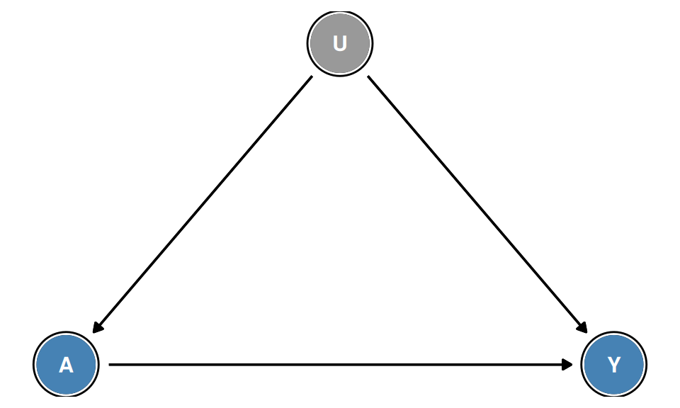
When the only common cause of \(A\) and \(Y\) is an unmeasured variable \(U\) (shown in gray), there is no measured set that satisfies the backdoor criterion. Standard adjustment methods cannot identify the causal effect without additional assumptions (e.g., instrumental variables, Chapter 16).
Unmeasured confounding:
Unmeasured confounding is the central challenge in observational causal inference. The assumption of “no unmeasured confounders” (conditional exchangeability given measured \(L\)) is untestable from observed data alone.
Strategies to address unmeasured confounding include:
- Sensitivity analysis: quantify how much an unmeasured confounder would need to change conclusions
- Negative controls: use outcome or exposure controls to detect unmeasured confounders
- Instrumental variable methods (Chapter 16): exploit exogenous variation in treatment assignment
- Difference-in-differences and fixed effects (Chapter 21): exploit longitudinal data structure
NoteFine Point 7.1: Do Not Adjust for Descendants of Treatment
A fundamental rule for constructing valid adjustment sets is: never include a descendant of treatment \(A\) in the adjustment set.
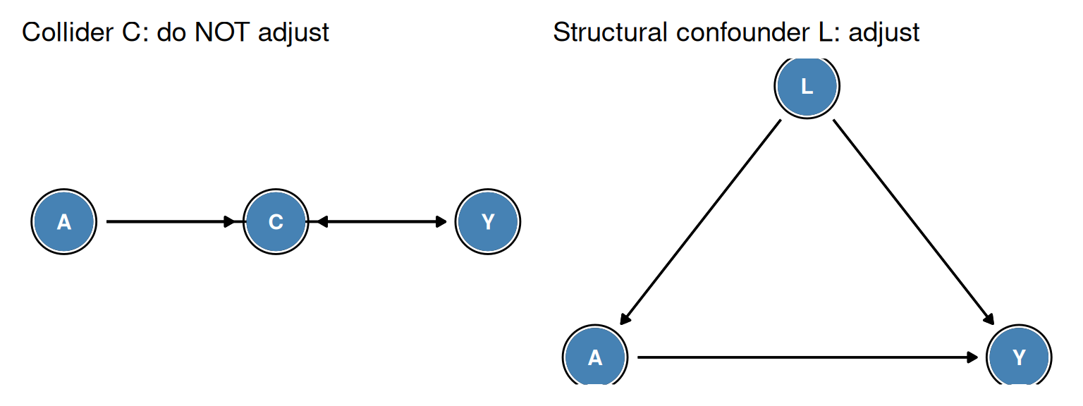
Why not? There are two distinct ways that adjusting for a post-treatment variable \(C\) (a descendant of \(A\)) can introduce bias:
Blocking part of the causal effect: If \(A \to C \to Y\) (so \(C\) is a mediator), conditioning on \(C\) removes part of the causal effect we are trying to estimate. We would estimate only the direct effect \(A \to Y\), not the total effect through \(C\).
Collider stratification bias: If \(A \to C \leftarrow U\) and \(U \to Y\) (so \(C\) is a collider on the path \(A \to C \leftarrow U \to Y\)), conditioning on \(C\) opens this previously blocked path and introduces a spurious association between \(A\) and \(Y\) via \(U\), even if \(U\) is unmeasured.
The second scenario is particularly insidious because the bias may not be obvious without drawing the causal diagram. The practical implication: when selecting variables to include in the adjustment set, first verify using the causal diagram that no candidate variable is a descendant of \(A\).
4 7.4 Confounding and Confounders (pp. 85–87)
The term confounder is commonly used in epidemiology to refer to a variable that should be adjusted for to eliminate confounding. However, the traditional criteria used to identify confounders differ from the structural (DAG-based) definition—and the two do not always agree.
4.1 The Traditional Epidemiological Criteria
In the traditional approach, a variable \(C\) is labeled a confounder of the \(A\)–\(Y\) association if it satisfies three criteria:
- \(C\) is associated with treatment \(A\)
- \(C\) is a risk factor for outcome \(Y\) among the unexposed (\(A = 0\))
- \(C\) is not on the causal pathway from \(A\) to \(Y\) (i.e., \(C\) is not a mediator)
These criteria are assessed from the data (criteria 1 and 2) and from prior knowledge (criterion 3).
4.2 Limitations of the Traditional Criteria
The traditional criteria have two important limitations:
Problem 1: A variable can satisfy all three criteria without being a structural confounder.
If \(C\) is a collider on a non-causal path between \(A\) and \(Y\) (e.g., \(A \to C \leftarrow Y\)), then \(C\) may be associated with both \(A\) and \(Y\) in some data sets yet is not on any backdoor path. Including \(C\) in the adjustment set could introduce collider stratification bias rather than removing confounding.
Problem 2: A structural confounder may fail one of the traditional criteria.
A variable \(L\) that opens a backdoor path from \(A\) to \(Y\) might fail criterion 1 (not associated with \(A\) in the data) if its effects on \(A\) and \(Y\) cancel in a specific population. In that population, adjusting for \(L\) is still required to eliminate structural confounding, but the traditional criteria would not flag it as a confounder.
Why the discrepancy matters:
The traditional approach of testing whether \(C\) is associated with \(A\) and \(Y\) and then deciding whether to adjust can lead to:
- Over-adjustment: Adjusting for colliders or mediators because they are associated with both \(A\) and \(Y\)
- Under-adjustment: Failing to adjust for structural confounders whose effects happen to cancel in the observed data
- Selection bias through collider adjustment: Stratifying on \(C = c\) when \(C\) is a collider opens the backdoor path and introduces bias
The DAG-based approach avoids these pitfalls by relying on causal structure rather than associations.
NoteFine Point 7.2: Limitations of Association-Based Confounder Criteria
The traditional association-based criteria for confounding are population-dependent: a variable \(L\) may satisfy criteria 1 and 2 in one population but not in another, even though the causal structure is identical. This means the decision about whether \(L\) is a “confounder” depends on the study population, not on the underlying causal mechanism.
In contrast, the structural (DAG-based) definition is population-independent: if \(L\) opens a backdoor path in the causal diagram, it is a structural confounder regardless of the population distribution.
This distinction has practical implications. When planning a study, one should identify the structural confounders using subject-matter knowledge and causal diagrams—not by testing associations in the current dataset. Adjusting for structural confounders is necessary to eliminate confounding bias across all populations satisfying the assumed causal structure.
5 7.5 Single-World Intervention Graphs (pp. 87–89)
The causal diagrams introduced in Chapter 6 represent relationships among observed variables (\(A\), \(L\), \(Y\), etc.). They do not directly represent counterfactual variables (\(Y^a\), \(L^a\), etc.). Single-World Intervention Graphs (SWIGs), developed by Richardson and Robins (2014), extend causal diagrams to include counterfactual variables explicitly.
5.1 Constructing a SWIG
A SWIG for the intervention \(A = a\) is obtained from the original causal diagram by the following operation:
-
Split each treatment node \(A\) into two parts:
- The fixed intervention value \(a\) (the value to which \(A\) is set by the intervention)
- The natural value \(A\) (the random variable representing what treatment the individual would have received in the absence of intervention)
- All arrows into \(A\) now point to the natural value \(A\); all arrows out of \(A\) now originate from the fixed value \(a\).
- Each child of \(A\) in the original DAG becomes a counterfactual variable (e.g., \(Y\) becomes \(Y^a\)).
The key result is that in the SWIG, counterfactual independence can be read off using d-separation, just as ordinary independence is read from a standard DAG.
5.2 What SWIGs Add
Standard DAGs allow us to determine which variables to adjust for (via the backdoor criterion) but cannot directly show that \(Y^a \perp\!\!\!\perp A \mid L\), because \(Y^a\) is not a node in the DAG. SWIGs resolve this by making counterfactual variables explicit:
- The d-separation statement \(Y^a \perp\!\!\!\perp A \mid L\) in the SWIG directly implies conditional exchangeability
- This equivalence provides a graphical justification for identification by standardization
Historical note:
SWIGs were introduced by Richardson and Robins (2014) as a formal framework for representing counterfactuals in causal diagrams. They unify the potential outcomes framework (Chapters 1–5) with the causal diagrams framework (Chapter 6) by constructing a single graph in which both observed and counterfactual variables appear.
Notation:
In SWIG notation, each treatment node \(A\) is written as \(a \mid A\) (read: “intervention value \(a\) given natural value \(A\)”). The counterfactual \(Y^a\) is written simply as \(Y^a\) or sometimes \(Y(a)\).
Beyond exchangeability:
SWIGs also provide a graphical representation of more complex counterfactual independence conditions, including those arising in time-varying treatment settings (Part III of the textbook). For example, in longitudinal settings, SWIGs can be used to represent the sequential exchangeability conditions needed to identify dynamic treatment regimes.
For most purposes in this textbook, standard DAGs combined with the backdoor criterion are sufficient. SWIGs provide an additional layer of rigor for readers interested in the formal connections between the potential outcomes framework and the graphical framework.
6 Summary
This chapter examined confounding in depth, providing both an intuitive numerical example and a formal structural definition.
Key concepts:
Confounding is present when the crude (marginal) association between \(A\) and \(Y\) differs from the average causal effect. Structurally, confounding exists when at least one backdoor path from \(A\) to \(Y\) is open.
Confounding = lack of marginal exchangeability: \(Y^a \not\perp\!\!\!\perp A\). The treated and untreated groups have different distributions of potential outcomes.
Conditional exchangeability (\(Y^a \perp\!\!\!\perp A \mid L\)) can restore identifiability when \(L\) satisfies the backdoor criterion. Under conditional exchangeability and positivity, the causal effect is identified by standardization.
The backdoor criterion provides a graphical sufficient condition for valid adjustment. A set \(L\) satisfies the criterion if it (i) contains no descendants of \(A\) and (ii) blocks all backdoor paths from \(A\) to \(Y\).
Structural vs. traditional confounders: The traditional association-based criteria for confounders can disagree with the structural (DAG-based) definition—either flagging colliders as confounders (causing harm from adjustment) or missing structural confounders. The DAG approach is preferred.
SWIGs embed counterfactual variables in a causal diagram and provide a graphical proof of conditional exchangeability whenever the backdoor criterion is satisfied.
Looking ahead:
- Chapter 8 examines selection bias—another structural source of bias arising from conditioning on colliders (or their descendants)
- Chapter 9 examines measurement bias—bias arising from imperfect measurement of \(A\), \(Y\), or \(L\)
- Chapters 12–15 present methods for adjusting for confounding: IP weighting, standardization, g-estimation, and outcome regression
Confounding bias is the central challenge in observational causal inference. This chapter has provided the structural tools needed to identify which variables to adjust for (the backdoor criterion) and the formal justification for why that adjustment works (conditional exchangeability, proved graphically via SWIGs).
7 References
Hernán, Miguel A, and James M Robins. 2020. Causal Inference: What If. Chapman & Hall/CRC. https://miguelhernan.org/whatifbook.