Chapter 6: Graphical Representation of Causal Effects
So far we have used potential outcomes to represent causal effects. In this chapter we use causal diagrams—directed acyclic graphs (DAGs)—to represent causal relations. Causal diagrams encode our qualitative assumptions about the causal structure of the problem and allow us to determine when association equals causation, and which variables need to be adjusted for to eliminate confounding.
This chapter is based on Hernán and Robins (2020, chap. 6, pp. 59–76).
1 6.1 Causal Diagrams (pp. 59–61)
A causal diagram is a directed acyclic graph (DAG) in which:
- Each node (vertex) represents a variable
- Each directed edge (arrow) from node \(V\) to node \(W\) represents a direct causal effect of \(V\) on \(W\)
- There are no cycles: following the arrows, you can never return to a starting node
1.1 The Main Example
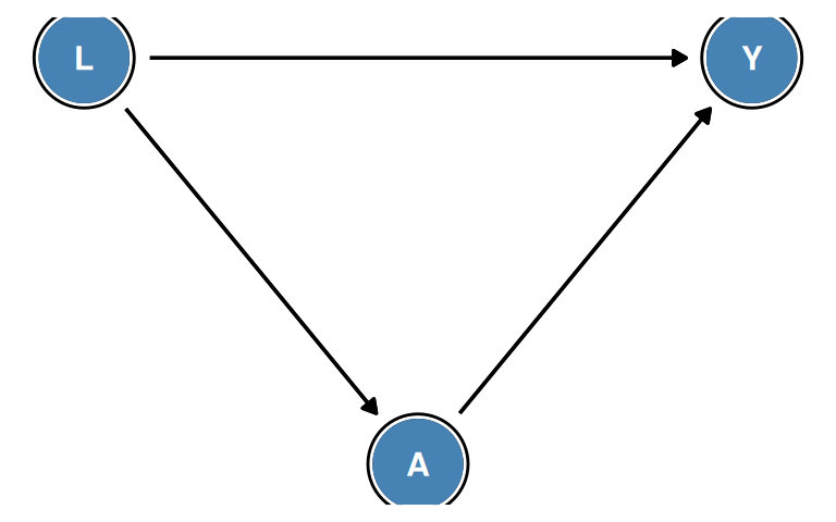
Consider a study of the causal effect of treatment \(A\) on outcome \(Y\), where \(L\) is a measured variable that causes both \(A\) and \(Y\). The structural equations are:
\[L = f_L(U_L)\] \[A = f_A(L,\, U_A)\] \[Y = f_Y(L,\, A,\, U_Y)\]
where \(U_L\), \(U_A\), and \(U_Y\) are mutually independent unmeasured background variables. The corresponding causal diagram is:
1.2 DAG Terminology
For a node \(W\) in a causal diagram:
- A parent of \(W\) is any node with a direct arrow into \(W\)
- A child of \(W\) is any node that \(W\) has a direct arrow into
- An ancestor of \(W\) is any node from which \(W\) is reachable by following arrows
- A descendant of \(W\) is any node reachable from \(W\) by following arrows
- A path between two nodes is any sequence of nodes connected by edges (arrows), regardless of direction
In Figure 6.1: \(L\) is a parent of \(A\) and a parent of \(Y\); \(A\) is a child of \(L\); \(Y\) is a descendant of \(L\) via two paths (\(L \to Y\) directly, and \(L \to A \to Y\)).
1.3 What DAG Arrows Represent
The presence of an arrow \(V \to W\) encodes the assumption that \(V\) has a direct causal effect on \(W\) (i.e., not entirely mediated by other variables explicitly shown in the graph).
The absence of an arrow between \(V\) and \(W\) (with no directed path from \(V\) to \(W\)) encodes the assumption that \(V\) has no direct causal effect on \(W\), given the other variables in the graph. This is a substantive causal assumption that must be justified by subject-matter knowledge.
What DAGs do and do not represent:
- Do represent: qualitative causal structure (which variables directly cause which)
- Do not represent: magnitude, direction, or functional form of effects
- Do not represent: effect modification (heterogeneity of effects across subgroups)
Why acyclic? DAGs do not allow feedback loops (e.g., \(A \to Y \to A\)). For dynamic settings with feedback, longitudinal DAGs or other frameworks are needed (see Part III of the textbook).
Unmeasured common causes: In Figure 6.1, we assume \(U_L\), \(U_A\), \(U_Y\) are mutually independent. If they were not independent — for instance, if \(U_A\) and \(U_Y\) were correlated — we would need to add an unmeasured common cause node connecting \(A\) and \(Y\), representing unmeasured confounding.
2 6.2 Causal Diagrams and Marginal Independence (pp. 61–64)
Causal diagrams encode information about which variables are marginally independent (independent unconditionally, before conditioning on any variable). We can read this information directly from the graph structure.
2.1 Open and Blocked Paths
A path between two nodes \(V\) and \(W\) is either open or blocked:
- A path is blocked if it contains a collider node — a node where two arrowheads meet on the path: \(\cdots \to C \leftarrow \cdots\)
- A path is open if it contains no collider (all intermediate nodes are non-colliders)
Two variables are marginally associated if and only if there is at least one open path between them.
d-separation:
The formal criterion for reading independence from a DAG is called d-separation. Two variables \(X\) and \(Y\) are d-separated by a conditioning set \(Z\) if all paths between \(X\) and \(Y\) are blocked given \(Z\). Under the Markov condition (which holds in any NPSEM with mutually independent \(U\) variables), d-separation implies conditional independence in the observed data.
Why colliders block paths marginally:
In an NPSEM, the collider \(C\) has independent causes \(A\) and \(Y\) (via their \(U\) variables). Without any conditioning, \(C\) is irrelevant to the association between \(A\) and \(Y\) — they have no shared cause and do not affect each other directly. The path through \(C\) is blocked.
Markov condition: In the NPSEM, each variable is independent of its non-descendants given its parents. This property is encoded in the DAG and is what allows us to use d-separation to determine independence.
3 6.3 Causal Diagrams and Conditional Independence (pp. 64–68)
Conditioning on a variable — by stratifying, restricting, or including it in a regression — can change independence relationships. Whether conditioning on a variable opens or blocks a path depends on whether that variable is a collider or a non-collider on the path.
3.1 Three Fundamental Path Structures
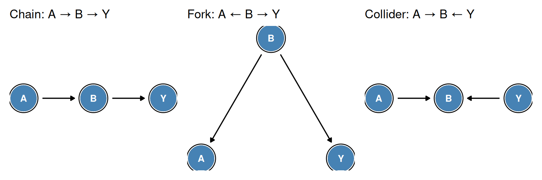
1. Chain: \(A \rightarrow B \rightarrow Y\)
- Marginally: \(A\) and \(Y\) are associated (open path \(A \to B \to Y\))
- Conditional on \(B\): \(A\) and \(Y\) are independent — conditioning on the intermediate variable \(B\) blocks the path
2. Fork: \(A \leftarrow B \rightarrow Y\)
- Marginally: \(A\) and \(Y\) are associated (open path through common cause \(B\))
- Conditional on \(B\): \(A\) and \(Y\) are independent — conditioning on the common cause \(B\) blocks the non-causal association
3. Collider: \(A \rightarrow B \leftarrow Y\)
- Marginally: \(A\) and \(Y\) are independent (path blocked by collider \(B\))
- Conditional on \(B\): \(A\) and \(Y\) are dependent — conditioning on a collider opens the previously blocked path
3.2 Collider Stratification Bias
Collider stratification bias is a subtle and important source of spurious association that arises from conditioning on a common effect of two variables.
Collider bias is pervasive in epidemiology:
- Berkson’s bias: Selecting cases and controls from a hospital creates a collider; diseases that are independent in the general population appear associated among hospitalized patients
- Healthy worker effect: Restricting to employed workers (whose employment is a common effect of health status and occupational exposure) induces a spurious association
- Survivorship bias: Among survivors of some condition, factors affecting survival appear spuriously associated
Descendants of colliders:
Conditioning on a descendant of a collider also partially opens the path, though with weaker bias. Any variable affected by both \(A\) and \(Y\) (or by a cause of \(A\) and a cause of \(Y\)) is potentially a collider or descendant of one.
Key practical principle: Do NOT adjust for variables that are downstream (descendants) of both treatment and outcome. This applies to selection into studies, loss to follow-up, or other post-treatment variables.
3.3 D-separation Rules (Summary)
The complete rules for determining whether a path is open or blocked after conditioning on a set \(Z\):
| Node type on path | \(B \notin Z\) (not conditioned on) | \(B \in Z\) (conditioned on) |
|---|---|---|
| Non-collider (chain or fork) | Open | Blocked |
| Collider | Blocked | Open |
Two variables are d-separated given \(Z\) if every path between them is blocked given \(Z\). D-separated variables are (conditionally) independent in any distribution generated by the NPSEM.
4 6.4 Positivity and Structural Causal Models (pp. 68–69)
4.1 Non-Parametric Structural Equation Models
Causal diagrams and their associated structural equations constitute non-parametric structural equation models (NPSEMs). The NPSEM framework provides a rigorous basis for defining counterfactual quantities from the observed data structure.
Given the structural equations \(L = f_L(U_L)\), \(A = f_A(L, U_A)\), \(Y = f_Y(L, A, U_Y)\) with \(U_L\), \(U_A\), \(U_Y\) mutually independent, the counterfactual outcome \(Y^a\) is formally defined as:
\[Y^a = f_Y\bigl(L,\, a,\, U_Y\bigr)\]
That is, \(Y^a\) is the value \(Y\) would take if we intervened to set \(A = a\), leaving all other structural equations (including those for \(L\) and the \(U\) variables) unchanged. This corresponds to Pearl’s do-operator: \(Y^a \equiv Y \,\mathrm{do}(A=a)\).
4.2 Positivity in Structural Causal Models
The positivity assumption requires that every individual has a positive probability of receiving each treatment level:
\[\Pr[A = a \mid L = l] > 0 \quad \text{for all } a \text{ and all } l \text{ with } \Pr[L = l] > 0\]
In structural equation terms, positivity requires that the function \(f_A(L, U_A)\) is not deterministic — no value of \(L\) should completely determine the treatment assignment \(A\).
Structural positivity violations occur when \(L\) deterministically forces \(A\) to a particular value. In these strata, the counterfactual \(Y^a\) cannot be identified from observational data regardless of sample size.
Random positivity violations occur when, by chance, certain \((A, L)\) combinations do not appear in the finite sample, even though they have positive probability in the population.
Why positivity matters for the NPSEM:
When \(\Pr[A = a \mid L = l] = 0\) for some \(l\), we observe no individuals with treatment \(a\) in stratum \(L = l\). We cannot therefore identify the counterfactual \(Y^a\) in that stratum from observational data. The causal effect is then not identifiable using standard methods (IP weighting, standardization, etc.) — a situation captured formally by the positivity assumption.
Consistency revisited:
In the NPSEM framework, the consistency assumption \(Y = Y^A\) follows directly from the structural equations: when \(A = a\) is actually assigned, \(Y = f_Y(L, A, U_Y) = f_Y(L, a, U_Y) = Y^a\). Consistency violations (e.g., multiple versions of treatment) correspond to a situation where the node \(A\) in the DAG actually represents several distinct interventions, each potentially yielding different outcomes.
5 6.5 A Structural Classification of Bias (pp. 69–73)
Causal diagrams provide a structural classification of the biases that may affect causal estimates. Three main types arise from the structure of the causal diagram.
5.1 Confounding Bias
Confounding is present when there is an open backdoor path from treatment \(A\) to outcome \(Y\).
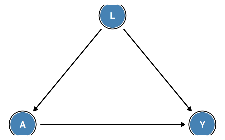
5.2 The Backdoor Criterion
Minimal sufficient adjustment sets:
Multiple sets may satisfy the backdoor criterion. A minimal sufficient adjustment set is one from which no variable can be removed while still satisfying the criterion. The R package dagitty enumerates minimal sufficient adjustment sets automatically.
Avoiding over-adjustment:
- Adjusting for a mediator (a descendant of \(A\) on a causal path to \(Y\)) blocks part of the causal effect — this is over-adjustment
- Adjusting for a collider introduces collider stratification bias
- Adjusting for a descendant of a collider partially introduces this bias
5.3 Selection Bias
Selection bias arises when the analysis conditions on a variable \(C\) that is a collider (or ancestor/descendant of a collider) on a path between \(A\) and \(Y\).
Structural representation:
\[A \longrightarrow C \longleftarrow Y\]
Restricting the analysis to individuals with \(C = 1\) (e.g., individuals selected into the study) opens the path \(A \to C \leftarrow Y\) and induces a spurious association between \(A\) and \(Y\).
Connection to collider stratification bias:
Selection bias is collider stratification bias applied to the selection mechanism. The “collider” is a variable related to study participation, follow-up completion, or analysis inclusion, and both \(A\) (or a cause of \(A\)) and \(Y\) (or a cause of \(Y\)) affect it.
Common examples:
- Loss to follow-up affected by both treatment and outcome
- Case-control studies where hospital admission depends on both exposure and disease
- Analysis restricted to survivors when survival depends on treatment and outcome
Chapter 8 covers selection bias in detail with specific examples.
5.4 Measurement Bias
Measurement bias (information bias) occurs when a variable is measured imperfectly. In the causal diagram, we distinguish:
- \(A\): the true (unmeasured or imperfectly measured) treatment
- \(A^*\): the observed (potentially error-prone) measurement of treatment
The structural relationship is \(A \to A^*\): the true value generates the measurement, with additional unmeasured factors \(U_{A^*}\) affecting the measurement.
Structural representation:
\[A \longrightarrow Y \qquad A \longrightarrow A^*\]
Using \(A^*\) in place of \(A\) produces a biased estimate of the causal effect of \(A\) on \(Y\).
Differential vs. non-differential measurement error:
- Non-differential (classical): \(A^* = f(A, U_{A^*})\) where \(U_{A^*}\) is independent of \(Y\) and \(L\) — typically attenuates estimates toward the null
- Differential: \(A^* = f(A, U_{A^*})\) where \(U_{A^*}\) is correlated with \(Y\) or its causes — can bias in either direction
Measurement error in confounders:
Measuring \(L\) imperfectly (using \(L^*\) instead of \(L\)) creates residual confounding: after adjusting for \(L^*\), the backdoor path \(A \leftarrow L \to Y\) is only partially blocked, and confounding bias remains.
Chapter 9 covers measurement bias in detail.
6 6.6 The Structure of Effect Modification (pp. 73–76)
6.1 Effect Modification in Causal Diagrams
Effect modification (heterogeneity of treatment effects) occurs when the causal effect of \(A\) on \(Y\) differs across levels of another variable \(V\). Standard DAGs, however, cannot directly represent effect modification.
A DAG with \(V \to Y\) and \(A \to Y\) is compatible with:
- No effect modification: the \(A \to Y\) effect is the same for all values of \(V\)
- Effect modification: the \(A \to Y\) effect varies across levels of \(V\)
Both cases have identical qualitative structure. The DAG encodes only the presence of causal effects (which variables cause which), not their magnitude or heterogeneity.
Why DAGs cannot encode effect modification:
Effect modification is a quantitative (or distributional) feature of the structural equations. A DAG specifies that \(Y = f_Y(L, A, U_Y)\) but makes no claim about whether \(f_Y\) involves an \(A \times V\) interaction term. Two different NPSEMs — one with and one without effect modification — are represented by the same DAG if they share the same qualitative causal structure.
Frameworks that can encode effect modification:
Extensions of the DAG framework, such as Single World Intervention Graphs (SWIGs) (Richardson and Robins, 2014) and annotated DAGs, can explicitly represent counterfactual quantities and some aspects of effect modification, but these are beyond the scope of this chapter.
6.2 Confounders, Effect Modifiers, and Both
A variable \(V\) can play different roles with respect to the \(A \to Y\) effect:
- Confounder: opens a backdoor path (\(V \to A\), \(V \to Y\)) — must adjust for \(V\) to remove bias
- Effect modifier: the \(A \to Y\) effect varies by \(V\) — should stratify by \(V\) to fully characterize effects
- Both: must adjust for \(V\) (confounding) and stratify (modification)
- Neither: \(V\) is unrelated to the \(A \to Y\) causal structure
6.3 Identifying Effect Modification
Because DAGs cannot directly represent effect modification, we must assess it empirically:
- First, ensure the causal effect is identified within each stratum of \(V\) (using the backdoor criterion or other identification strategies)
- Estimate stratum-specific causal effects \(\text{E}{\left[Y^{a=1} - Y^{a=0} \mid V = v\right]}\) for each level \(v\)
- Compare effect estimates across strata: if they differ, effect modification is present
Effect modification and interaction:
Chapter 5 defined additive interaction between two treatments \(A\) and \(E\) using the interaction contrast \(\text{IC} = \text{E}{\left[Y^{a=1,e=1}\right]} - \text{E}{\left[Y^{a=1,e=0}\right]} - \text{E}{\left[Y^{a=0,e=1}\right]} + \text{E}{\left[Y^{a=0,e=0}\right]}\). Effect modification of the \(A \to Y\) effect by \(V\) corresponds to the case where \(V\) plays the role of \(E\), but one where \(V\) is not itself a treatment under consideration — it simply describes a subgroup characteristic.
Scale-dependence:
Effect modification is scale-dependent (Chapter 4). The \(A \to Y\) effect may be modified by \(V\) on the risk difference scale but not on the risk ratio scale. The DAG cannot distinguish between these cases; the scale of modification must be specified separately.
7 Summary
This chapter introduced causal diagrams (DAGs) as graphical tools for encoding causal assumptions and determining the identifiability of causal effects from observed data.
Key concepts:
DAGs and NPSEMs: A DAG represents a non-parametric structural equation model. Each variable \(V_k\) satisfies \(V_k = f_k(\mathrm{pa}(V_k), U_k)\) with mutually independent background variables \(U_k\)
Marginal independence: Two variables are marginally independent if all paths between them are blocked (d-separated). A collider on a path blocks it marginally.
-
Three fundamental path structures:
- Chain (\(A \to B \to Y\)): Conditioning on \(B\) blocks the path
- Fork (\(A \leftarrow B \to Y\)): Conditioning on \(B\) blocks the path
- Collider (\(A \to B \leftarrow Y\)): Conditioning on \(B\) opens the path — collider stratification bias
Positivity and NPSEMs: The positivity assumption requires that treatment assignment is not deterministic given \(L\). Counterfactuals \(Y^a\) are formally defined via the structural equations as \(Y^a = f_Y(L, a, U_Y)\)
-
Structural classification of bias:
- Confounding: open backdoor path from \(A\) to \(Y\) (common cause not conditioned on)
- Selection bias: conditioning on a collider (common effect) on a path between \(A\) and \(Y\)
- Measurement bias: using an imperfect measure \(A^*\) instead of the true \(A\)
Backdoor criterion: A set \(L\) satisfying (i) no descendant of \(A\) in \(L\), (ii) \(L\) blocks all backdoor paths — adjusting for \(L\) eliminates confounding
Effect modification: Standard DAGs encode qualitative structure only; effect modification cannot be read from the DAG and must be assessed empirically
Practical workflow:
- Draw a DAG based on subject-matter knowledge before analyzing data
- Identify all backdoor paths from \(A\) to \(Y\)
- Find a sufficient adjustment set satisfying the backdoor criterion
- Adjust for that set (IP weighting, standardization, regression)
- Do not adjust for colliders, mediators, or descendants of treatment
Software:
- R package
dagitty: draw DAGs, enumerate adjustment sets, test d-separation - R package
ggdag: visualize DAGs (used in this chapter) - Web interface: dagitty.net
Limitations of DAGs:
- Require qualitative causal assumptions justified by subject-matter knowledge
- Unmeasured common causes must be added explicitly as \(U\) nodes; otherwise assumed absent
- Cannot represent dynamic feedback (cycles)
- Cannot encode effect modification or effect magnitudes
- Cannot represent interference between individuals
Looking ahead:
- Chapter 7: Detailed treatment of confounding — definition, assessment, and adjustment
- Chapter 8: Selection bias — conditioning on common effects
- Chapter 9: Measurement bias — error in exposures and confounders
- Chapters 11–15: Estimation methods — IP weighting, g-formula, propensity scores
8 References
Hernán, Miguel A, and James M Robins. 2020. Causal Inference: What If. Chapman & Hall/CRC. https://miguelhernan.org/whatifbook.